Credit Risk Model using ML
1. Problem Statement:
The aim is to create a machine learning model that can precisely segregate customers into classes of credit based on past financial data and other pertinent borrower characteristics, including income, credit score, and loan details. The likelihood that a borrower will fail on a loan should be estimated by the model, allowing it to determine the risk of lending to them. Such models can help financial institutions identify and measure their total risk exposure, set appropriate risk limits, and make informed investment decisions.
2. Solution Work Flow:

3. Challenges Faced:
One of the biggest challenges in credit risk modelling is the limited availability of relevant and reliable data. Credit risk models require historical data on loan performance, default rates, and economic indicators to accurately assess the likelihood of default.
Challenges include data availability, data quality, complex modelling, and regulatory compliance. Example: One common challenge faced by financial institutions is obtaining accurate and reliable data for credit risk modelling purposes.
How to approach a machine learning credit risk problem?
Detail Model Description:
1. There are two datasets. We need to solve the challenges that are faced by the bank during credit lending.
2. First dataset is (i) Internal bank dataset and second dataset is (ii) Cibil external dataset.
3. The target variable is Approved_Flag, which contains 4 categories ['P2', ‘P1’, ‘P3’, ‘P4’], segregating the customer into classes for giving credit. P1 is the category where the bank can easily give credit to that customer, whereas P4 is the category where it is not a good idea to give credit to that customer, as it can increase the NPA accounts (non-Performing assets) of the bank.
4. To find associations between numerical and numerical columns, we will perform the VIF test (variance inflation factor). Reject columns whose p value is greater than a particular threshold.
5. For feature selection, we will perform chi2 square test and Anova test, since the target column is multi-class categorical column.
6. By checking the p_value of each column with respect to the target variable, we can decide if it’s statistically significant or not.
7. made two models. One without credit score and another with credit score.
8. It is observed that the accuracy of model without credit score feature has dramatically decreases.
9. Without credit score, the accuracy is 77% and with credit score, the accuracy is 99%.
Important feature descriptions for the datasets:
Bank Dataset:

Cibil Dataset:

Important Notes from both datasets:
1. The shape of bank internal dataset is (51336, 26).
2. The shape of cibil dataset is (51336, 62).
3. The common column in both datasets is PROSPECTID, which is unique ID for each customer.
4. The value “-99999” in both datasets are null values.
5. We will remove all the null values if data lost is less than 20% of the total dataset.
6. Total trade lines is total number of accounts of a customer.
Unique Values from categorical columns:

After performing all statistical tests (i.e., the chi square, VIF, and Anova tests), it was found that 43 columns were important out of 82.
[
  'Age_Newest_TL', 'Age_Oldest_TL', 'Approved_Flag', 'CC_enq_L12m', 'CC_Flag', 'CC_TL', 'EDUCATION',
  'first_prod_enq2', 'GENDER', 'GL_Flag', 'HL_Flag', 'Home_TL', 'last_prod_enq2', 'MARITALSTATUS',
  'max_recent_level_of_deliq', 'NETMONTHLYINCOME', 'num_dbt_12mts', 'num_dbt', 'num_deliq_6_12mts',
  'num_lss', 'num_std_12mts', 'num_sub_12mts', 'num_sub_6mts', 'num_sub', 'num_times_60p_dpd',
  'pct_CC_enq_L6m_of_ever', 'pct_PL_enq_L6m_of_ever', 'pct_tl_closed_L12M', 'pct_tl_closed_L6M',
  'pct_tl_open_L6M', 'PL_enq_L12m', 'PL_Flag', 'PL_TL', 'recent_level_of_deliq', 'Secured_TL',
  'time_since_recent_enq', 'time_since_recent_payment', 'Time_With_Curr_Empr', 'Tot_Missed_Pmnt',
  'Tot_TL_closed_L12M', 'Unsecured_TL', 'enq_L3m', 'Other_TL',
]
Data Visualisation:
Age Distribution Graph

The data distribution of this dataset is mostly spread between the age group of 20 and 40.
Age of Oldest loan/Trade Line account (In Months)

Time since recent enquiry (In Months)

Credit Score Distribution

Most of the data distribution in credit score column is spread between 660 and 700, which fall under P2 category and that’s why the majority of the category in target column is P2 category only.
90 percentile Monthly Income Distribution

This column illusrate that the salary income of the majority of people falls between $20k and $35k. It can be observed that the bank is mainly targeting those people whose income is under $50,000 per month
Marital Status Distribution Graph

This column indicates that 73.1% of people who are applying for the loan are married.
Education Distribution Graph

The Graduate and 12th pass population contribute significantly to the dataset
Gender Distribution Graph:

Gender wise, the dataset shows that 88.7% of those applying for loans are male, or we can say that the bank is targeting male candidates more as compared to female candidates.
Last Product Enquiry Graph

Previous loans taken by the people in this dataset is other loan or consumer loans (such as furniture loan, fridge loans, etc).
First Product Enquiry Graph

Distribution of Target Variable Categories

60% of the people in the dataset fall under the P2 category for loan approval.
Relationship of Target variable with other features
Minimum, Maximum and median value of Credit Score for each category

The min and max credit score in P3 category is 489 and 776 respectively. This range indicates that the P3 category creates a lot of ambiguity for the model to predict the output accurately. For P1 and P2 categories, it is easier for the model to predict as it ranges from (701, 809) and (689, 700), respectively.
Minimum, Maximum and median values of Age for each category

The minimum age for all the category is 21. The maximum age varies from 63 to 67. It can be observed that for P1 category, the median age is higher as compared to other categories and as the category decreases, the median age also decreases.
Observation of numerical and categorical columns with respect to the target variable, i.e. approved flag
1. P1 category range is (701–809)
2. P2 category range is (669–700)
3. P3 category range is (489–776)
4. P3 category of target variable is the most ambiguous category. This can be observed by looking at the credit score min and max value for P3 category, which range from 489 to 776, whereas in case of P2, they ranges from 669 to 701.
5. P3 being the most ambiguous category, causes the model decrease it’s accuracy to a significantly level.
6. The median age of those getting P1 category loans is a bit older than other categories. For example, the median age for the P1 category is 40, whereas for the P2 category it is 33, and for the P3 category it is 31. Therefore, it can be observed that as age increases, loan approval becomes easier.
Model Training:
We used ensemble techniques (bagging and boosting) to train the model. Mainly, we used random forest and XGBoost classifier for this classification problem. It is observed that XGboost classifier has better accuracy as compared to random forest classifier. With accuracy of 99%, with credit score feature included, XGBoost is the best ML algorithm for the dataset. However, when credit score feature is excluded, there is a significant drop in accuracy (76%).
When taking model without credit score feature, the following is the recall, precision and f1 score for all classes:

Hyperparameter Tuning:
Using BayesSearchCV, we got the best parameter for our XGBoost model. The parameters are:
{
  "alpha": 10,
  "colsample_bytree": 0.9,
  "learning_rate": 1.0,
  "max_depth": 3,
  "n_estimators": 100,
  "num_classes": 4,
  "objective": "multi:softmax",
}
With these parameters, accuracy increases to 78% when the model is trained without credit score column.
This is one of the many ways how financial institutions solve credit risk problems and decreases number of NPAs (non-performing assets) to maintain financial stability and profitability.